How to Upload a Csv File in R
Welcome! If you lot want to start diving into information science and statistics, then data frames, CSV files, and R will be essential tools for you. Let's meet how you can employ their amazing capabilities.
In this commodity, you volition learn:
- What CSV files are and what they are used for.
- How to create CSV files using Google Sheets.
- How to read CSV files in R.
- What Data Frames are and what they are used for.
- How to admission the elements of a information frame.
- How to change a data frame.
- How to add and delete rows and columns.
We will utilize RStudio, an open-source IDE (Integrated Evolution Environment) to run the examples.
Let's begin! ✨
🔹 Introduction to CSV Files
CSV (Comma-separated Values) files can exist considered one of the building blocks of data analysis because they are used to store data represented in the form of a tabular array.
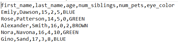
In this file, values are separated by commas to represent the dissimilar columns of the table, like in this example:
Nosotros will generate this file using Google Sheets.
🔸 How to Create a CSV File Using Google Sheets
Let's create your first CSV file using Google Sheets.
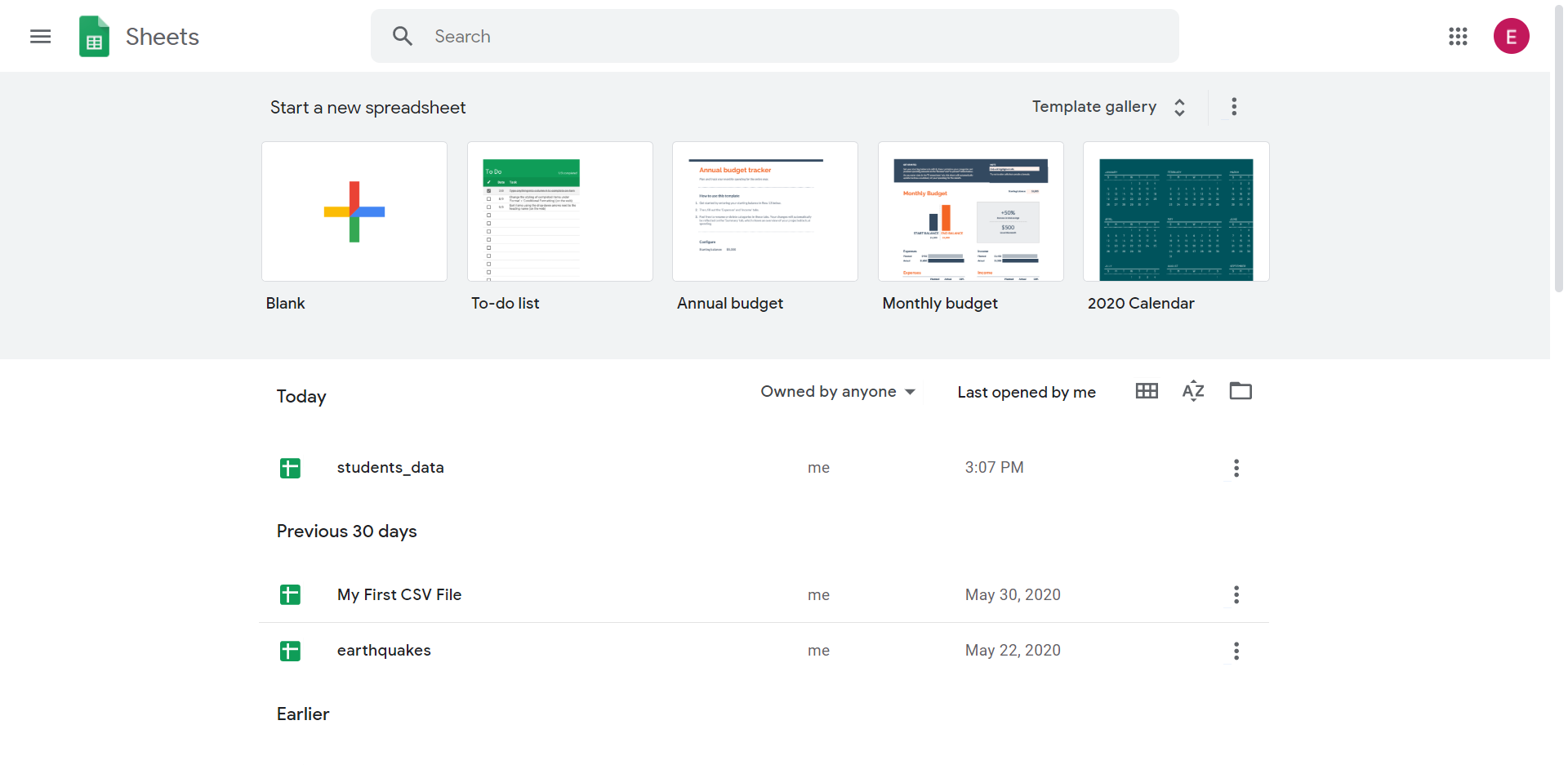
Pace ane: Go to the Google Sheets Website and click on "Go to Google Sheets":
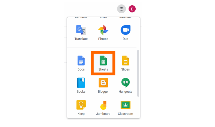
💡 Tip: You lot can access Google Sheets by clicking on the push button located at the top-right edge of Google'southward Home Page:

If nosotros zoom in, we see the "Sheets" button:
💡 Tip: To employ Google Sheets, you need to take a Gmail account. Alternatively, y'all can create a CSV file using MS Excel or another spreadsheet editor.
Y'all volition run into this panel:
Pace 2: Create a blank spreadsheet by clicking on the "+" button.
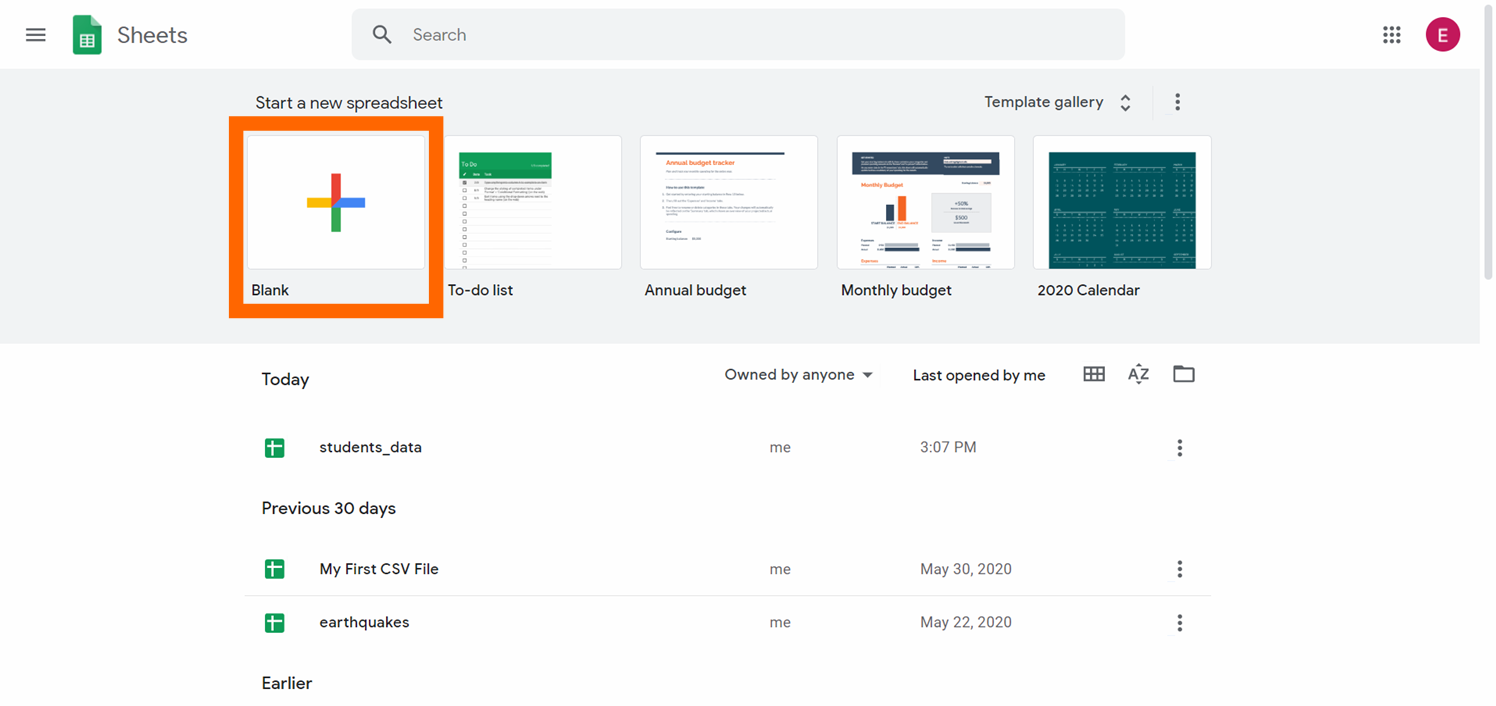
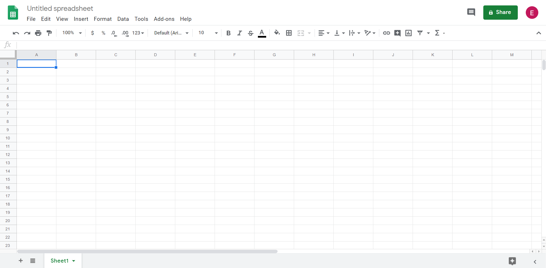
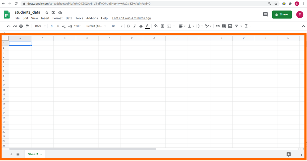
Now you lot have a new empty spreadsheet:
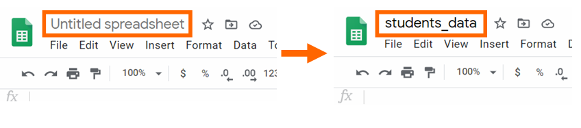
Step 3: Change the name of the spreadsheet to students_data. Nosotros will demand to use the proper name of the file to work with data frames. Write the new name and click enter to confirm the change.
Step 4: In the start row of the spreadsheet, write the titles of the columns.
When you import a CSV file in R, the titles of the columns are called variables. We will define half-dozen variables: first_name, last_name, age, num_siblings, num_pets, and eye_color, equally you tin can come across right here below:
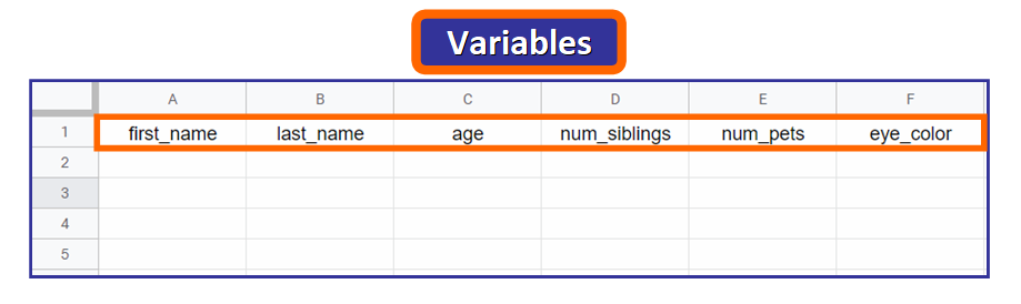
💡 Tip: Find that the names are written in lowercase and words are separated with an underscore. This is not mandatory, simply since you lot volition need to access these names in R, it's very common to use this format.
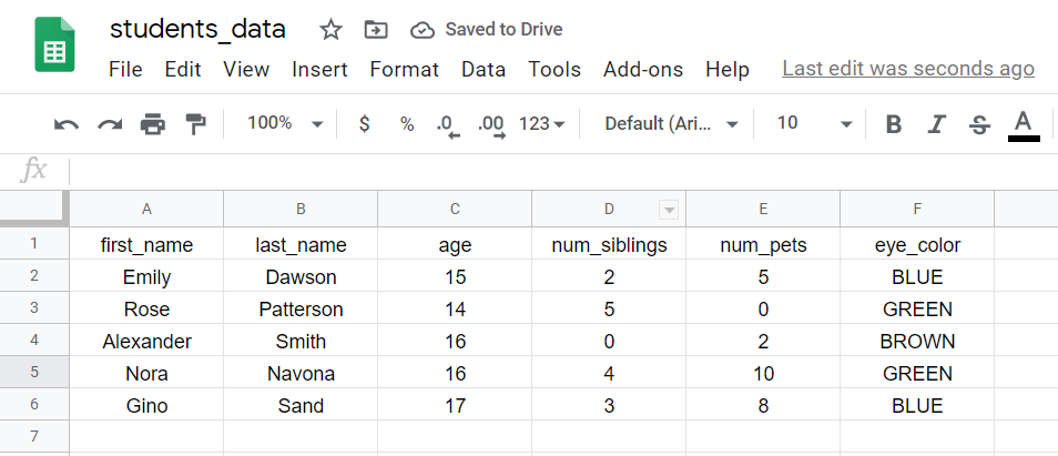
Step 5: Enter the data for each one of the columns.
When you lot read the file in R, each row is chosen an observation, and it corresponds to information taken from an individual, fauna, object, or entity that we collected data from.
In this case, each row corresponds to the information of a educatee:
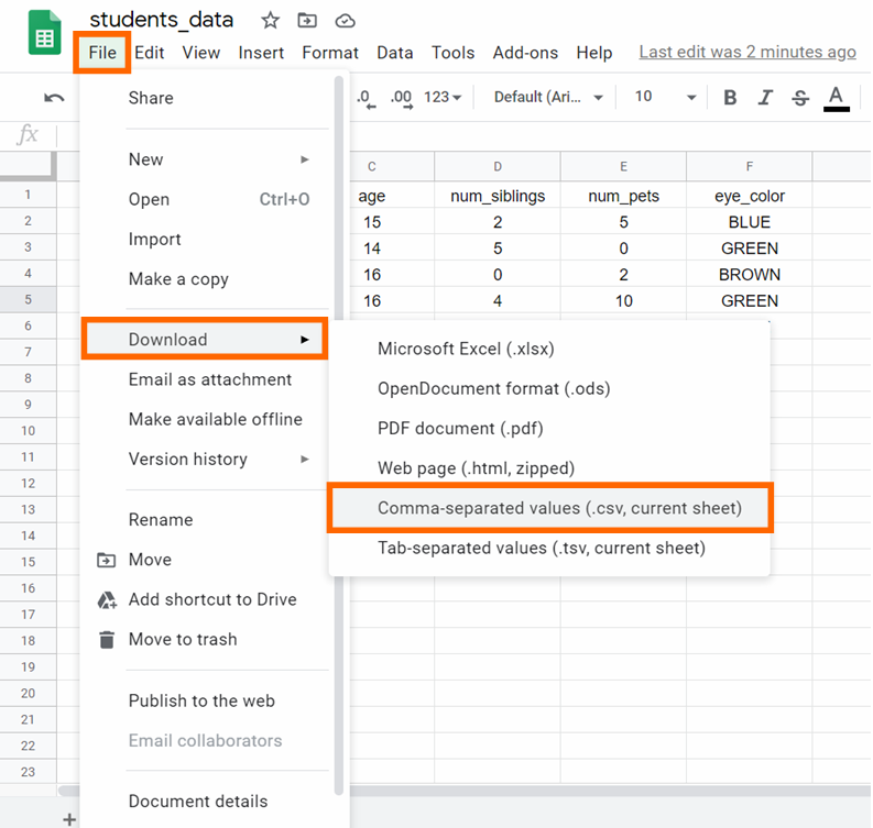
Step 6: Download the CSV file by clicking on File -> Download -> Comma-separated values, every bit you tin can see below:
Step 7: Rename the file CSV file. You will need to remove "Sheet1" from the default name because Google Sheet will automatically add this to the name of the file.

Slap-up work! Now you accept your CSV file and it'southward time to offset working with it in R.
🔹 How to Read a CSV file in R
In RStudio, the first pace earlier reading a CSV file is making certain that your current working directory is the directory where the CSV file is located.
💡 Tip: If this is not the case, you will need to use the full path to the file.
Change Current Working Directory
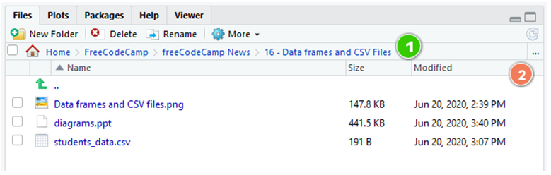
You can change your current working directory in this panel:
If we zoom in, you lot can run across the current path (1) and select the new one by clicking on the ellipsis (...) push button to the right (ii):
💡 Tip: Y'all tin also check your current working directory with getwd() in the interactive console.
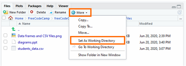
Then, click "More" and "Prepare As Working Directory".
Read the CSV File
Once you have your electric current working directory gear up, you can read the CSV file with this command:
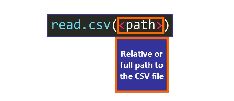
In R code, nosotros have this:
> students_data <- read.csv("students_data.csv") 💡 Tip: We assign it to the variable students_data to access the data of the CSV file with this variable. In R, nosotros can separate words using dots ., underscores _, UpperCamelCase, or lowerCamelCase.
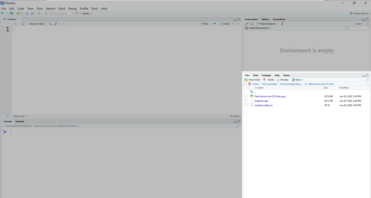
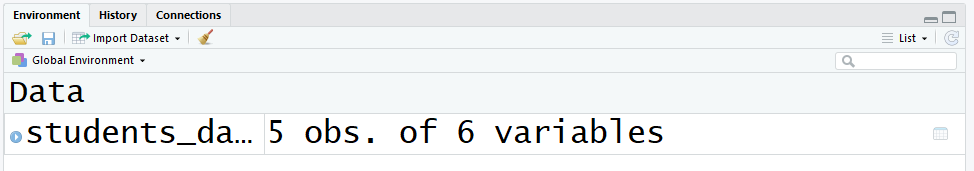
After running this command, you will see this in the meridian right panel:
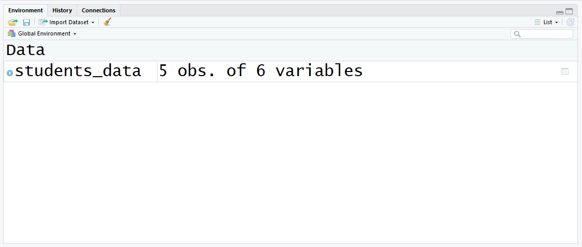
Now you take a variable defined in the environment! Let's run across what data frames are and how they are closely related to CSV files.
🔸 Introduction to Data Frames
Data frames are the standard digital format used to store statistical data in the class of a tabular array. When you read a CSV file in R, a data frame is generated.
Nosotros can confirm this by checking the type of the variable with the grade function:
> class(students_data) [1] "information.frame" It makes sense, right? CSV files comprise data represented in the grade of a tabular array and information frames correspond that tabular data in your lawmaking, so they are deeply connected.
If yous enter this variable in the interactive panel, you volition run into the content of the CSV file:
> students_data first_name last_name historic period num_siblings num_pets eye_color 1 Emily Dawson fifteen two 5 BLUE ii Rose Patterson 14 5 0 Greenish 3 Alexander Smith 16 0 2 BROWN 4 Nora Navona 16 4 10 GREEN 5 Gino Sand 17 3 8 BLUE More Information Nigh the Data Frame
You have several unlike alternatives to see the number of variables and observations of the data frame:
- Your get-go option is to await at the elevation right console that shows the variables that are currently divers in the environs. This information frame has v observations (rows) and 6 variables (columns):
- Another alternative is to use the functions
nrowandncolin the interactive console or in your programme, passing the data frame as argument. Nosotros get the same results: 5 rows and six columns.
> nrow(students_data) [1] 5 > ncol(students_data) [1] 6 - You can also see more information almost the data frame using the
strfunction:
> str(students_data) 'data.frame': 5 obs. of 6 variables: $ first_name : Factor w/ 5 levels "Alexander","Emily",..: 2 5 1 4 iii $ last_name : Cistron due west/ 5 levels "Dawson","Navona",..: one 3 5 2 4 $ age : int xv 14 xvi 16 17 $ num_siblings: int ii 5 0 4 3 $ num_pets : int v 0 2 10 eight $ eye_color : Factor w/ 3 levels "BLUE","BROWN",..: one iii 2 iii 1 This function (applied to a data frame) tells you lot:
- The number of observations (rows).
- The number of variables (columns).
- The names of the variables.
- The information types of the variables.
- More than information about the variables.
You can see that this part is really swell when y'all want to know more than about the data that yous are working with.
💡 Tip: In R, a "Factor" is a qualitative variable, which is a variable whose values correspond categories. For case, eye_color has the values "Blue", "Brown", "GREEN" which are categories, and so as you can see in the output of str above, this variable is automatically defined every bit a "factor" when the CSV file is read in R.
🔹 Information Frames: Key Operations and Functions
Now yous know how to meet more information nearly the data frame. But the magic of data frames lies in the amazing capabilities and functionality that they offer, so let's come across this in more than detail.
How to Access A Value of a Data Frame
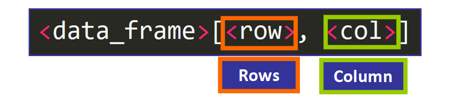
Information frames are like matrices, so you can access individual values using ii indices surrounded by square brackets and separated by a comma to indicate which rows and which columns you lot would like to include in the effect, like this:
For example, if we want to access the value of eye_color (column 6) of the fourth educatee in the data (row 4):
We demand to utilise this command:
> students_data[4, vi] 💡 Tip: In R, indices start at one and the first row with the names of the variables is not counted.
This is the output:
[1] GREEN Levels: BLUE Chocolate-brown GREEN You can run across that the value is "GREEN". Variables of type "factor" have "levels" that represent the different categories or values that they can take. This output tells us the levels of the variable eye_color.
How to Access Rows and Columns of a Data Frame
Nosotros can also use this syntax to access a range of rows and columns to get a portion of the original matrix, similar this:
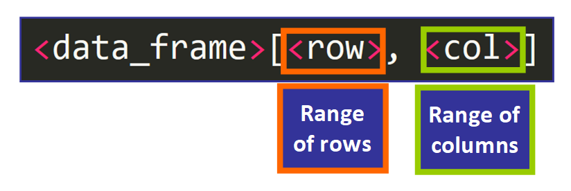
For example, if we desire to get the historic period and number of siblings of the third, fourth, and fifth student in the listing, we would apply:
> students_data[3:5, 3:4] age num_siblings 3 16 0 4 sixteen 4 5 17 3 💡 Tip: The basic syntax to ascertain an interval in R is <start>:<end>. Notation that these indices are inclusive, so the third and fifth elements are included in the example above when nosotros write 3:5.
If we want to become all the rows or columns, nosotros simply omit the interval and include the comma, like this:
> students_data[3:five,] first_name last_name age num_siblings num_pets eye_color 3 Alexander Smith 16 0 2 Chocolate-brown four Nora Navona 16 4 10 GREEN 5 Gino Sand 17 three eight Blueish We did not include an interval for the columns after the comma in students_data[iii:v,], so we go all the columns of the data frame for the iii rows that we specified.
Similarly, nosotros can get all the rows for a specific range of columns if we omit the rows:
> students_data[, 1:three] first_name last_name age 1 Emily Dawson fifteen 2 Rose Patterson 14 3 Alexander Smith xvi 4 Nora Navona 16 v Gino Sand 17 💡 Tip: Notice that you still need to include the comma in both cases.
How to Access a Column
At that place are three ways to access an unabridged column:
- Pick #1: to access a column and return it equally a data frame, you can utilise this syntax:
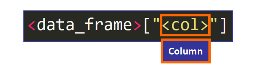
For instance:
> students_data["first_name"] first_name 1 Emily 2 Rose 3 Alexander four Nora five Gino - Option #2: to go a cavalcade as a vector (sequence), you lot can use this syntax:
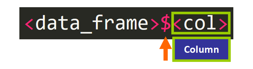
💡 Tip: Discover the utilize of the $ symbol.
For instance:
> students_data$first_name [ane] Emily Rose Alexander Nora Gino Levels: Alexander Emily Gino Nora Rose - Option #3: You can also use this syntax to get the column every bit a vector (meet below). This is equivalent to the previous syntax:
> students_data[["first_name"]] [one] Emily Rose Alexander Nora Gino Levels: Alexander Emily Gino Nora Rose How to Filter Rows of a Data Frame
You tin filter the rows of a data frame to get a portion of the matrix that meets certain conditions.
For this, we use this syntax, passing the condition as the get-go chemical element within square brackets, then a comma, and finally leaving the second chemical element empty.
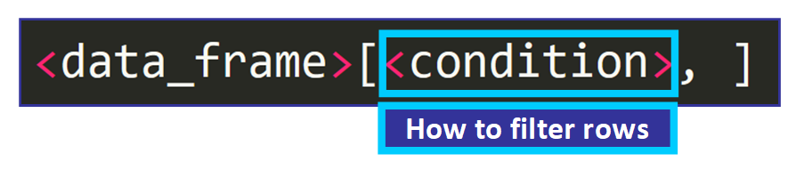
For example, to get all rows for which students_data$age > 16, we would use:
> students_data[students_data$age > sixteen,] first_name last_name age num_siblings num_pets eye_color 5 Gino Sand 17 iii 8 BLUE Nosotros get a data frame with the rows that run across this status.
Filter Rows and Choose Columns
Y'all can combine this condition with a range of columns:
> students_data[students_data$age > 16, three:vi] age num_siblings num_pets eye_color v 17 3 8 Bluish We get the rows that encounter the condition and the columns in the range 3:vi.
🔸 How to Change Information Frames
You tin can modify private values of a data frame, add columns, add rows, and remove them. Let'south see how yous can practice this!
How to Change A Value
To modify an private value of the information frame, you need to use this syntax:
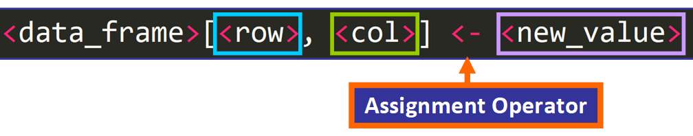
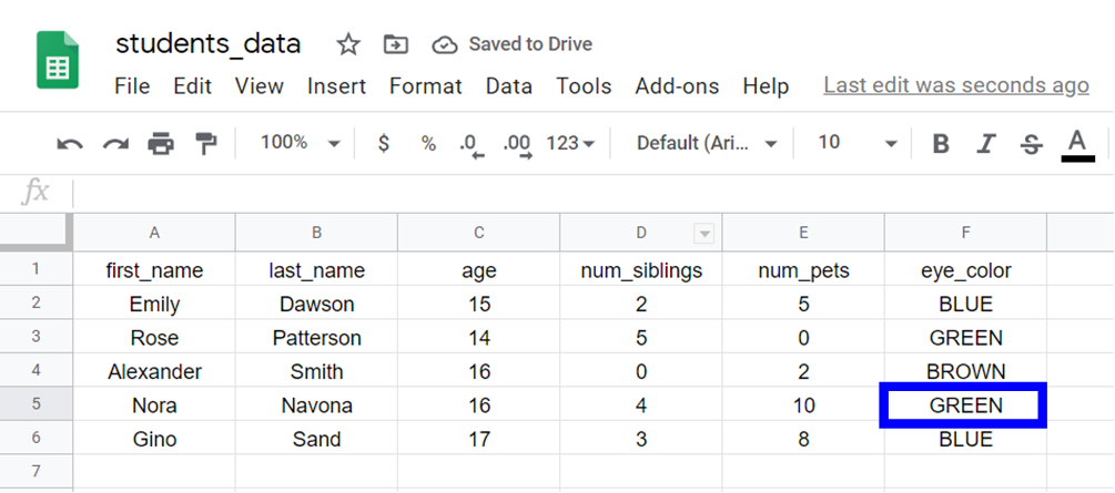
For example, if we want to change the value that is currently at row 4 and column 6, denoted in blue right here:
Nosotros need to employ this line of lawmaking:
students_data[iv, 6] <- "BROWN" 💡 Tip: You can as well use = every bit the assignment operator.
This is the output. The value was inverse successfully.
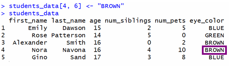
💡 Tip: Remember that the first row of the CSV file is not counted as the get-go row considering it has the names of the variables.
How to Add together Rows to a Data Frame
To add together a row to a information frame, you lot need to apply the rbind role:
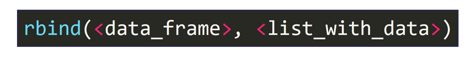
This part takes 2 arguments:
- The data frame that y'all want to modify.
- A list with the data of the new row. To create the listing, you can use the
listing()function with each value separated by a comma.
This is an example:
> rbind(students_data, list("William", "Smith", 14, 7, three, "Dark-brown")) The output is:
first_name last_name age num_siblings num_pets eye_color i Emily Dawson 15 two v Blueish 2 Rose Patterson 14 5 0 GREEN three Alexander Smith sixteen 0 2 Brown 4 Nora Navona 16 4 10 BROWN 5 Gino Sand 17 3 eight Blueish 6 <NA> Smith 14 7 3 Dark-brown But wait! A warning message was displayed:
Warning message: In `[<-.factor`(`*tmp*`, ri, value = "William") : invalid factor level, NA generated And observe the starting time value of the sixth row, it is <NA>:
6 <NA> Smith xiv 7 iii BROWN This occurred because the variable first_name was defined automatically as a cistron when we read the CSV file and factors have fixed "categories" (levels).
You cannot add a new level (value - "William") to this variable unless you read the CSV file with the value FALSE for the parameter stringsAsFactors, every bit shown beneath:
> students_data <- read.csv("students_data.csv", stringsAsFactors = Faux) 
Now, if nosotros attempt to add this row, the data frame is modified successfully.
> students_data <- rbind(students_data, listing("William", "Smith", xiv, 7, 3, "Dark-brown")) > students_data first_name last_name historic period num_siblings num_pets eye_color 1 Emily Dawson fifteen 2 5 Bluish ii Rose Patterson 14 5 0 GREEN 3 Alexander Smith 16 0 2 BROWN 4 Nora Navona sixteen four 10 GREEN 5 Gino Sand 17 3 viii Blueish 6 William Smith 14 seven three BROWN 💡 Tip: Annotation that if yous read the CSV file again and assign it to the same variable, all the changes made previously will be removed and you volition encounter the original data frame. You need to add this argument to the first line of code that reads the CSV file and then brand changes to it.
How to Add Columns to a Data Frame
Adding columns to a data frame is much simpler. You need to use this syntax:

For example:
> students_data$GPA <- c(four.0, 3.5, 3.ii, 3.15, two.9, 3.0) 💡 Tip: The number of elements has to be equal to the number of rows of the data frame.
The output shows the information frame with the new GPA column:
> students_data first_name last_name age num_siblings num_pets eye_color GPA 1 Emily Dawson fifteen 2 five Blueish 4.00 2 Rose Patterson 14 five 0 Dark-green 3.50 iii Alexander Smith 16 0 2 Brown 3.20 4 Nora Navona 16 iv 10 GREEN 3.fifteen 5 Gino Sand 17 3 8 Blueish 2.90 half dozen William Smith 14 7 3 BROWN iii.00 How to Remove Columns
To remove columns from a data frame, you lot need to use this syntax:
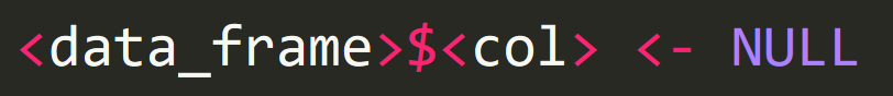
When y'all assign the value Nada to a cavalcade, that column is removed from the data frame automatically.
For example, to remove the historic period column, nosotros apply:
> students_data$age <- NULL The output is:
> students_data first_name last_name num_siblings num_pets eye_color GPA 1 Emily Dawson 2 v BLUE 4.00 two Rose Patterson 5 0 GREEN iii.fifty 3 Alexander Smith 0 2 BROWN 3.xx 4 Nora Navona 4 x Dark-green iii.15 five Gino Sand iii 8 BLUE 2.90 vi William Smith 7 3 BROWN three.00 How to Remove Rows
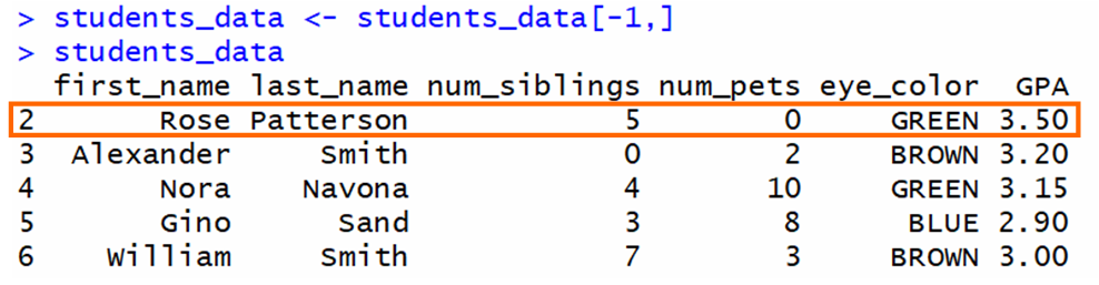
To remove rows from a data frame, you can use indices and ranges. For example, to remove the kickoff row of a data frame:

The [-1,] takes a portion of the information frame that doesn't include the first row. And then, this portion is assigned to the same variable.
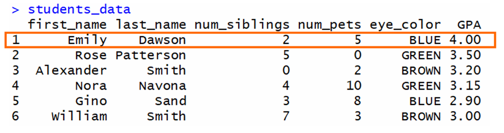
If nosotros have this data frame and nosotros desire to delete the get-go row:
The output is a data frame that doesn't include the first row:
In full general, to remove a specific row, you need to use this syntax where <row_num> is the row that yous want to remove:

💡 Tip: Notice the - sign before the row number.
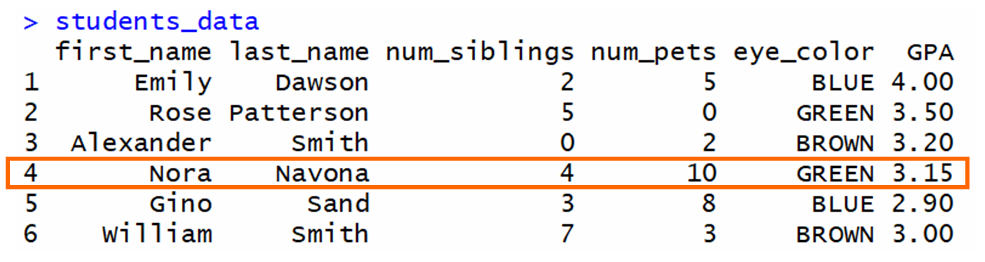
For example, if nosotros want to remove row 4 from this data frame:
The output is:
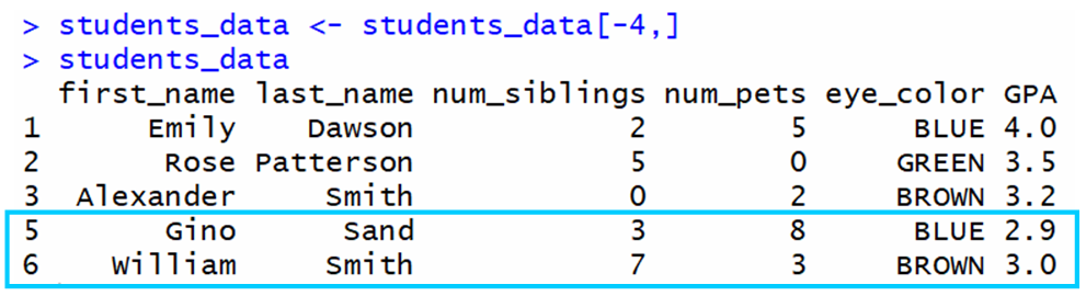
As you can see, row four was successfully removed.
🔹 In Summary
- CSV files are Comma-Separated Values Files used to represent data in the form of a tabular array. These files can be read using R and RStudio.
- Data frames are used in R to represent tabular data. When yous read a CSV file, a data frame is created to store the information.
- Y'all can admission and modify the values, rows, and columns of a data frame.
I actually hope that you liked my commodity and plant it helpful. Now yous can work with data frames and CSV files in R.
If you liked this article, consider enrolling in my new online grade "Introduction to Statistics in R - A Practical Arroyo "
Learn to lawmaking for free. freeCodeCamp'southward open source curriculum has helped more than 40,000 people get jobs as developers. Get started
Source: https://www.freecodecamp.org/news/how-to-work-with-data-frames-and-csv-files-in-r/
0 Response to "How to Upload a Csv File in R"
Post a Comment